Density estimation

Introduction

• Last week we looked a Bayes decision theory
• Nice theoretically, but assumes knolwedge about probablity desnity distribution.
• This is rarely available, so how to we proceed.
• Estimate densities from data!

• In this lecture we will cover:
  • Mixture modeling
  • Non-parametric density estimation
    • K nearest neighbor approach
  • K nearest neighbor classifier

---

Mixture models

• Take a look at the following data:

import numpy as np
import matplotlib.pyplot as plt

# Set random seed for reproducibility
np.random.seed(42)

# Generate data samples from three normal distributions
mean1, cov1 = [2, 3], [[1.5, 0.5], [0.5, 1]]  # Mean and covariance for distribution 1
mean2, cov2 = [6, 5], [[1, -0.3], [-0.3, 1.2]]  # Mean and covariance for distribution 2
mean3, cov3 = [4, 1], [[0.8, 0.2], [0.2, 0.5]]  # Mean and covariance for distribution 3

data1 = np.random.multivariate_normal(mean1, cov1, 300)
data2 = np.random.multivariate_normal(mean2, cov2, 300)
data3 = np.random.multivariate_normal(mean3, cov3, 300)

# Combine the data for visualization
data = np.vstack((data1, data2, data3))

plt.figure(figsize=(7, 5))
plt.scatter(data[:, 0], data[:, 1])
plt.show()

How can we handle this "mix" of distributions?

• Model the unknown density $p(\mathbf{x})$ via a linear combination of density functions:
• $p(\mathbf{x})=\sum_{j=1}^{J}p(\mathbf{x}|j)P_j$
• where
  • $\sum_{j=1}^{J}P_j=1$ and $\int p(\mathbf{x}|j) d\mathbf{x}=1$

What are the implications of this mix of models?

• Assumes that each sample $\mathbf{x}$ may be "drawn" from any of the $J$ distributions.
• What is the problem here?

How to perform the modeling?

• First step:
  • Assume a parametric form $p(\mathbf{x}|j;\boldsymbol{\theta})$
• Need to find the unkown parameters $\theta$ and $P_j$ for $j=1,\cdots,J$.
• What would be your first idea?

How to perform the modeling?

• First idea:
  • Maximize the likelihood function -> $\prod_k p(\mathbf{x}_k|j;\boldsymbol{\theta}, P_1, P_2, \cdots , P_J)$
• Problem:
  • Unknown parameters enter the maximization task in a nonlinear fashion.

The Expectation Maximisation (EM) - algorithm

• The EM algorithm is one of the most widely used methods for local maximum likelihood estiamte of parameters.
• Ideally suited to handle incomplete data settings.
• Let $\mathbf{y}\in Y \subseteq \mathcal{R}^m$ denote the complete data samples.
  • Probability density function $p_y(\mathbf{y};\boldsymbol{\theta})$, with unkown parameters $\boldsymbol{\theta}$.
• Problem:
  • The $y\text{'s}$ cannot be directly observed.
  • Instead, we observe: $\mathbf{x}=g(\mathbf{y})\in X_{ob} \subseteq \mathcal{R}^l$, where $l<m$.
  • Probablity density function of $\mathbf{x}$ denoted $p_x(\mathbf{x};\boldsymbol{\theta})$

The Expectation Maximisation (EM) - algorithm

• We have a many-to-one-mapping. ->
• Let $Y(\mathbf{x})\subseteq Y$, that is, the subset of all the $y\text{'s}$. corresponding to a specific $\mathbf{x}$.
• Then, the probablity density of the incomplete data is:
  • $p_x(\mathbf{x};\boldsymbol{\theta})=\int_{Y(\mathbf{x})}p_y(\mathbf{y};\boldsymbol{\theta})d\mathbf{y}$.

The Expectation Maximisation (EM) - algorithm

• Maximum likelihood estimate of $\theta$ is found by:
• $\hat{\theta}_m : \sum_k \frac{\partial \ln(p_y(y_k; \theta))}{\partial \theta} = \mathbf{0}$
• Problem:
  • We do not have the $y\text{'s}$.
• EM-algorithm maximises the expcations of the likelihood function, conditioned on the observed samples and the current estimate of $\theta$.
• Consists of two iterative steps:
  • E-step -> expectation step.
  • M-step -> maximization step

The E and M step

• E-step:
  • Calculate $Q(\theta; \theta^{(t)}) = \mathbb{E}\left\{ \sum_k \ln p_y(y_k; \Theta) | X, \theta^{(t)} \right\}$
• M-step:
  • Update $\theta^{(t+1)}$ by maximising $Q(\theta; \theta^{(t)})$
  • i.e. $\theta^{(t+1)} : \frac{\partial Q(\theta; \theta^{(t)})}{\partial \theta} = 0$

Practical considerations

• Need a starting point for our unknown parameters.
  • Many smart ways to find this starting point, but still a challenging aspect.
• When do we stop iterating? ->

Application to mixture modelling

• Consider a case with complete data.
  • Joint events $(\mathbf{x}_k), j_k$.
• Applying Bayes rule gives:
  • $p_y(\mathbf{x}, j_k;\theta)=p_y(\mathbf{x}| j_k;\theta)P_{jk}$.
• Assuming independence between samples, the log-likeligood is:
  • $L(\theta)=\sum_{k=1}^{N} \ln(p_y(\mathbf{x}| j_k;\theta)P_{jk})$

Application to mixture modelling

• Let $\mathbf{P} = \begin{bmatrix} P_1, P_2, \ldots, P_J \end{bmatrix}^T$ and the complete parameters: $$ \boldsymbol{\Theta} = \begin{bmatrix} \boldsymbol{\theta}^T, \mathbf{P}^T \end{bmatrix}^T $$

• Hence the E-step: $$ Q(\boldsymbol{\Theta}; \boldsymbol{\Theta}^{(t)}) = \mathbb{E} \left\{ \sum_{k=1}^N \ln \left( p(\mathbf{x}_k | j_k; \boldsymbol{\Theta}) P_{j_k} \right) \right\} $$

Application to mixture modelling - the Gaussian case

• Eg., for Gaussian with $\Sigma_j = \sigma_j^2 I$:

• $P_j$, $\mu_j$ and $\sigma_j$ are unknown.

• E-step: $$ p(x_k | j_k; \Theta) = \frac{1}{(2\pi \sigma_j^2)^{1/2}} \exp\left( -\frac{\|x_k - \mu_j\|^2}{2\sigma_j^2} \right) $$

• Thus, $$ Q(\Theta, \Theta^{(t)}) = \sum_{k=1}^N \sum_{j=1}^J P(j | x_k, \Theta^{(t)}) \left( -\frac{1}{2} \ln \sigma_j - \frac{1}{2\sigma_j^2} \|x_k - \mu_j\|^2 + \ln P_j \right) $$

Application to mixture modelling - the Gaussian case

• M-step: $$ \mu_j^{(t+1)} = \frac{\sum_{k=1}^N P(j | \mathbf{x}_k; \Theta^{(t)}) \, \mathbf{x}_k}{\sum_{k=1}^N P(j | \mathbf{x}_k; \Theta^{(t)})} $$

$$ \sigma_j^2 (t+1) = \frac{\sum_{k=1}^N P(j | \mathbf{x}_k; \Theta^{(t)}) \, \|\mathbf{x}_k - \mu_j^{(t+1)}\|^2}{\sum_{k=1}^N P(j | \mathbf{x}_k; \Theta^{(t)})} $$

Application to mixture modelling - the Gaussian case

$$ P_j(t+1) = \frac{1}{N} \sum_{k=1}^N P(j | \mathbf{x}_k, \Theta^{(t)}) $$

Where $$ P(j | \mathbf{x}_k, \Theta^{(t)}) = \frac{p(\mathbf{x}_k | j; \Theta^{(t)}) P_j(t)}{p(\mathbf{x}_k; \Theta^{(t)})} $$

and $$ p(\mathbf{x}k; \Theta^{(t)}) = \sum{j=1}^J p(\mathbf{x}_k

import numpy as np
import matplotlib.pyplot as plt
from scipy.stats import multivariate_normal

# Generate synthetic data from three Gaussians
np.random.seed(42)
N = 300
means_true = np.array([[2, 3], [6, 5], [4, 1]])
covs_true = [np.array([[1.5, 0.5], [0.5, 1]]),
             np.array([[1, -0.3], [-0.3, 1.2]]),
             np.array([[0.8, 0.2], [0.2, 0.5]])]
data = np.vstack([
    np.random.multivariate_normal(means_true[i], covs_true[i], N//3)
    for i in range(3)
])

# Initialization
K = 3
N_total = data.shape[0]
np.random.seed(0)
#means = data[np.random.choice(N_total, K, replace=False)]
means = np.random.rand(K, 2) * 10
covs = [np.eye(2) for _ in range(K)]
weights = np.ones(K) / K

def e_step(data, means, covs, weights):
    resp = np.zeros((data.shape[0], K))
    for k in range(K):
        resp[:, k] = weights[k] * multivariate_normal.pdf(data, mean=means[k], cov=covs[k])
    resp /= resp.sum(axis=1, keepdims=True)
    return resp

def m_step(data, resp):
    Nk = resp.sum(axis=0)
    means = np.dot(resp.T, data) / Nk[:, None]
    covs = []
    for k in range(K):
        diff = data - means[k]
        cov = np.dot(resp[:, k] * diff.T, diff) / Nk[k]
        covs.append(cov)
    weights = Nk / data.shape[0]
    return means, covs, weights

# Run EM for 10 iterations and plot selected iterations
iterations_to_plot = [1, 2, 5, 10]
plt.figure(figsize=(20, 4))
for i in range(1, 11):
    resp = e_step(data, means, covs, weights)
    means, covs, weights = m_step(data, resp)
    if i in iterations_to_plot:
        idx = iterations_to_plot.index(i)
        plt.subplot(1, 4, idx+1)
        plt.scatter(data[:, 0], data[:, 1], c=resp.argmax(axis=1), cmap='viridis', s=10)
        for k in range(K):
            plt.scatter(means[k, 0], means[k, 1], c='red', marker='x', s=100)
        plt.title(f'Iteration {i}')
plt.suptitle('EM Algorithm: Expectation and Maximization Steps')
plt.show()

import numpy as np
import matplotlib.pyplot as plt
from ucimlrepo import fetch_ucirepo
from sklearn.mixture import GaussianMixture

# fetch dataset 
iris = fetch_ucirepo(id=53)

# data (as pandas dataframes) 
X = iris.data.features.iloc[:, :2]
X_1_name = 'sepal length (cm)'
X_2_name = 'sepal width (cm)'
y = np.zeros(150)
y[50:100] = 1
y[100:150] = 2
y_names = iris.data.targets

number_of_components = [2,3,4, 5, 6]

plt.figure(1, figsize=(12, 3))
for counter, n_components_i in enumerate(number_of_components):
    gm = GaussianMixture(n_components=n_components_i, random_state=0).fit(X)
    plt.subplot(1, 5, counter+1)
    plt.scatter(X.iloc[:, 0], X.iloc[:, 1], c=y, cmap='viridis', edgecolor='k', s=50)
    plt.scatter(gm.means_[:, 0], gm.means_[:, 1], s=100, color='blue')
    plt.xlabel(X_1_name)
    plt.ylabel(X_2_name)
plt.tight_layout()
plt.show()

number_of_random_inits = range(3)

plt.figure(1, figsize=(12, 3))
for counter, _ in enumerate(number_of_random_inits):
    random_seed = np.random.randint(0, 100)
    gm = GaussianMixture(n_components=2, random_state=random_seed, init_params='random').fit(X)
    plt.subplot(1, 3, counter+1)
    plt.scatter(X.iloc[:, 0], X.iloc[:, 1], c=y, cmap='viridis', edgecolor='k', s=50)
    plt.scatter(gm.means_[:, 0], gm.means_[:, 1], s=100, color='blue')
    plt.xlabel(X_1_name)
    plt.ylabel(X_2_name)
plt.tight_layout()
plt.show()

K nearest neighbor density estimation

• Parzen estimation from last lecture:
  • Points are fixed and put "area" around point
• What happens if we reverse the roles?

samples = np.array([
    [1, 1.1], [1.3, 1.2], [0.7, 1.3],  # Spread out within the first cluster
    [4.5, 4.8], [4.8, 5.2],            # Spread out within the second cluster
    [7, 2.5],                          # Separate point moved closer
    [3.5, 6.5],                        # Separate point moved closer
    [8, 8.5]                           # Separate point moved closer
])

plt.figure(figsize=(8, 5))
plt.scatter(samples[:, 0], samples[:, 1], color='blue', s=100)
plt.show()

Nearest neighbor classification

• Can create powerful classification algorithms using nearest neighbors.
• Simple idea:
  • Step 1:
  • Step 2:
  • Step 3:
• A bit simplified:
  • What can go wrong above?
  • Limitations?

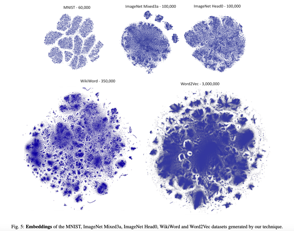
Recent advances to address computational burden - Faiss

• Faiss is a library for efficient similarity search.
• Github repository for Faiss.
• Example from Pezzotti et al., 2020k

Recent advances to address computational burden - Faiss

Programming exercises

Below are programming exercises assocaited with this lecture. These cell blocks are starting points that loads the data and prepares the problem such that you can get going with the implementation. There are also theoretical exercsies, but due to copyright we cannot shared them here. They will be made available in a private repository connected to the course.

Gaussian mixture modeling of Iris dataset

The code below loads the Iris dataset that we have looked at previously. Perform mixture modeling under the assumption of Gaussian distribution. Experiment with different number of components, initialization methods, and number of iterations.

import numpy as np
import matplotlib.pyplot as plt
from ucimlrepo import fetch_ucirepo

# fetch dataset 
iris = fetch_ucirepo(id=53)
  
# data (as pandas dataframes) 
X = iris.data.features.iloc[:, :2]
X_1_name = 'sepal length (cm)'
X_2_name = 'sepal width (cm)'
y = np.zeros(150)
y[50:100] = 1
y[100:150] = 2
y_names = iris.data.targets


plt.figure(1)
plt.scatter(X.iloc[:, 0], X.iloc[:, 1], c=y, cmap='viridis', edgecolor='k', s=50)
plt.xlabel(X_1_name)
plt.ylabel(X_2_name)
plt.show()

Non-linear classification with a NN classifier

The code below loads a classic synthetic machine learning dataset, the Two Moons dataset. This is a binary classification problem that is not solvable with a linear classifier (try one of your classifiers from previous notebooks and see for yourself.) Design a nearest neighbor classifier and see if you can tackle the Two Moons problem.

from sklearn.datasets import make_moons
X, y = make_moons(n_samples=200, noise=0.15, random_state=42)

plt.figure(1)
plt.scatter(X[:, 0], X[:, 1], c=y, cmap='viridis', edgecolor='k', s=50)
plt.show()